What is e-value?

A standard practice for assessing primary homology of a gene sequence is through local alignment (e.g., NCBI’s BLAST), in which an input sequence (the “query”) is matched against a particular sequence (the “hit”) in a database of sequences. The metric most commonly used to determine the significance of an alignment between a query and its hit is e-value. Given the ubiquity of this parameter, here is a short guide to explain what it is and how it’s used.

What is e-value?
E-value (short for expect value) is a calculation of the number of sequences in the database that are expected, by chance in a random search, to align equally or more significantly to the query than the hit that was found. It reflects the frequency that you will find an equal or better match in the database for your query sequence. In effect, e-value is an estimate of the hit to have been chosen due to random background noise.

What does the value mean, and what is the range of possible e-values?
An e-value of 1.0 means that you expect one sequence in the database to match the query as well or better than the hit you found. An e-value of 0.0 means zero sequences can/are expected to match as well or better; the closer the e-value is to zero, the more significant (and less of a potential false positive) the match is considered to be.

Although e-values can range from zero to theoretically infinity, most e-values will be a decimal between 0 and 1, represented by scientific notation (e.g., 1e-05 = 0.00001). Matches above 1.0 are most of the time not considered significant (the default cutoff for blastn, the most inclusive NCBI BLAST search, is 10.0). This does not mean that they are not potentially homologous sequences, just that a random search is expected to find multiple better candidates.

What goes into calculating e-value?
E-value = K*m*n*e^(-λ*S)
K,λ = constants based on scoring matrix; m,n = lengths of the two sequences; S = alignment score, which is calculated based on the alignment produced (incorporating matches, mismatches, gaps, etc).

Therefore, e-value is mostly dependent upon the length of the sequences, the size of the database, and the derived alignment score. This implies that shorter sequences, especially with lower complexity, are less likely to be matched significantly (and are often filtered out). Moreover, e-values derived from searches across databases of different size cannot be compared. An e-value of 6e-32 from a search against a small database is less significant than an e-value of 6e-32 from a large database; as the database grows, the likelihood of the presence of a truly homologous sequence grows in tandem, and consequently the likelihood of a false positive decreases.

Is an e-value the thing same as a p-value?
No. E-value is a frequency metric, whereas p-value is a probability metric. Though both metrics reflect the significance of the query-hit alignment, e-value represents the number of better alignments that are expected to occur by chance, while p-value represents the likelihood that the match in question occurred by chance. (In statistical terms, the e-value is a multiple testing correction of the p-value.)

NCBI uses e-value as its standard because it provides greater clarity and granularity; “it is easier to understand the difference between, for example, e-value of 5 and 10 than p-values of 0.993 and 0.99995.” Both can be used, but be aware of which you are using and why, because they represent different things.

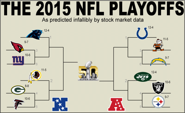
Using the stock market to predict the 2015 NFL season standings

Ah, early September. Shorter days, cooler weather, and the triumphant return of Professional HandEgg (aka “football”). Try as laymen and experts alike might, predicting football on a weekly basis is a notoriously difficult endeavor; predicting entire seasons is basically impossible. This is the case for a number of reasons: week to week variance is high, outcomes are dependent on the actions of no fewer than 44 individuals and upwards of 88 per game, and football is rife with irreducible error in the form of sample size–the season is only 16 games long, and the difference between 8 wins and 10 will always be extremely small. Oh, and the football gods are known to be cruel and unusual punishers; just ask Ricardo Lockette. But that’s beside the point.

So, given all of these limitations, how can we more reliably predict the NFL season? Well, rather than build complex models such as DVOA over at Football Outsiders, which are often based on the few reliable metrics that can be extracted from such a complex game, I thought to take a totally different approach. If sports are one of the hardest things to predict, why not try to predict them using data from the very hardest thing to predict: the stock market! In other words, why not take an even more difficult to predict arena and see if its data performs any better as a predictor?

Here’s how it works: for each team, I chose the largest publicly trading company within its state. (For states with multiple teams, I dipped into the second and third largest companies, and ordered based on those teams’ 2014 record.) This included companies such as Apple for the 49ers, Coca-Cola for the Falcons, etc. Unfortunately, the Broncos were represented by DISH network, not Papa John’s. For the Giants and Jets I used NY companies; for the Redskins I used DC companies; for the Chiefs, I used Missouri companies. These were chosen based on the most recently available public data, which ranged from 2012-2014. Here’s the table of companies for each team:

Team	Company
Arizona Cardinals	Freeport-McMoRan
Atlanta Falcons	Coca-Cola
Baltimore Ravens	Lockheed Martin
Buffalo Bills	JPMorgan Chase
Carolina Panthers	Bank of America
Chicago Bears	AbbVie
Cincinnati Bengals	Procter & Gamble
Cleveland Browns	Cardinal Health of Dublin
Dallas Cowboys	ExxonMobil
Denver Broncos	DISH Network
Detroit Lions	Dow Chemical
Green Bay Packers	Johnson Controls
Houston Texans	AT&T
Indianapolis Colts	Eli Lily and Company
Jacksonville Jaguars	Tech Data
Kansas City Chiefs	Express Scripts Holding
Miami Dolphins	World Fuel Services
Minnesota Vikings	3M
New England Patriots	Biogen Idec, Inc.
New Orleans Saints	CenturyLink
New York Giants	AIG
New York Jets	Citigroup
Oakland Raiders	Wells Fargo
Philadelphia Eagles	PNC Financial
Pittsburgh Steelers	Comcast
San Diego Chargers	Google
San Francisco 49ers	Apple
Seattle Seahawks	Microsoft
St. Louis Rams	Anheuser-Busch
Tampa Bay Buccaneers	Jabil Circuit
Tennessee Titans	FedEx
Washington Redskins	Capital One

Using MarketWatch stock charts, I recorded the weekly price of an individual stock for each corporation for the past 17 weeks. I then calculated percent difference in stock per week, and used that differential as a “score” for each team’s game on a weekly basis. Whoever’s score was greater earned a win — much like football itself! I implemented these data across all 256 games throughout the season, and generated final win-loss records for each team.

As an example, tonight’s game, Comcast (Steelers) will be defeated by Biogen Idec, Inc. (Patriots), with a score of +0.176% for Biogen to -0.021% for Comcast from May 15th to May 22nd. All the excitement of football sucked out and all the tedium of markets infused in. Sounds like a terrible idea and a complete waste of time, right? I agree!

Let’s get on with the results. Based on weekly stock data for the top public corporations in America, here are your 2015 NFL standings:

AFC East
1. New York Jets	12-4
2. Buffalo Bills	9-7
3. New England Patriots	7-9
4. Miami Dolphins	6-10
AFC North
1. Cleveland Browns	11-5
2. Pittsburgh Steelers	9-7
2. Baltimore Ravens	9-7
4. Cincinnati Bengals	6-10
AFC West
1. Oakland Raiders	10-6
2. San Diego Chargers	9-7
3. Denver Broncos	8-8
4. Kansas City Chiefs	7-9
AFC South
1. Indianapolis Colts	12-4
2. Houston Texans	9-7
3. Jacksonville Jaguars	6-10
4. Tennessee Titans	3-13
NFC East
1. Washington Redskins	11-5
2. New York Giants	10-6
3. Philadelphia Eagles	6-10
4. Dallas Cowboys	5-11
NFC North
1. Green Bay Packers	8-8
2. Detroit Lions	7-9
2. Chicago Bears	7-9
4. Minnesota Vikings	4-12
NFC West
1. Arizona Cardinals	9-7
1. San Francisco 49ers	9-7
3. St. Louis Rams	8-8
4. Seattle Seahawks	5-11
NFC South
1. Carolina Panthers	12-4
2. Atlanta Falcons	10-6
3. Tampa Bay Buccaneers	7-9
4. New Orleans Saints	5-11

Some observations:

• The New York Jets are tied for the best record in football! If not for an early September blowout by Andrew Luck and co., Gang Green would be sitting atop the AFC, presumably thanks to the unstoppable duo of Geno Smith and Brandon Marshall, a few weeks of jaw recovery notwithstanding. Who needs Rex?!
• In fact, this model seems to love the plucky underdog, particularly in the AFC, where the Raiders enjoy their first playoff berth since 2002, the Jets earn their first bye since the Bronze Age, and the Browns make the playoffs for the first time since man attained sapience. Unfortunately, fortune did not smile upon the unassuming teams in the 9-7 wild card logjam. Of the five teams who could have secured wild card spots, the Steelers and Chargers emerged, thanks to some head-to-head and divisional tiebreakers. After a brief absence, the Steelers thus return to the playoffs, shattering the dreams of less fortunate franchises like the Bills and the Texans. Sorry, Bills and Texans.
• A rough year for each member of last year’s Super Bowl XLIX, as the Patriots finish just under .500, and the Seahawks have an outright disastrous 5-11 year, setting them up for a top 5 draft pick. Who knew Kam Chancellor was the key to their success?
• Poor Jaguars and Titans. Even in a wacky simulation, they’re garbage.

• Over in the NFC, the East ended up being the exact opposite of last year’s standings, and probably the exact opposite of what you would expect this year. High expectations for the Cowboys and Eagles are shattered as both teams fell well short of the postseason. Dan Snyder has never been prouder as his plucky Potatoes emerge atop the division, securing a cushy bye and folk hero status for the eternally affable and beloved Mr. Snyder. The Kirk Cousins era starts with a bang!
• The Panthers build upon their wondrous season as the second team ever to clinch a division under .500 by winning the top seed in the conference. Meanwhile, the NFC North is a veritable tire fire, with the Packers emerging as 8-8 victors.
• I promise I did not cheat by having both New York teams make the playoffs. Which is exactly what a cheater would say…
• Finally, if nothing else, this should be solid affirmation that you should in no way under any circumstances use the least predictable thing on earth to predict the second least predictable thing on earth.

All that said, here’s the resulting playoff picture. Call your bookies now, before it’s too late! Happy football!

How to retrieve a set of sequences from within a FASTA file with Python

A common need in bioinformatics is to extract a subset of sequences from within a FASTA file. You might only want sequences from a particular taxon, sequences that were matched in a BLAST search, sequences that you chose by throwing a dart on a map of South America — the reasons are endless. Imagining a file with five nucleotide sequences labeled Seq1-Seq5, and that you only want odd numbered sequences, like so:

Original fasta file:	List of genes you want:	Desired output:
>Seq1 ACTGCGTATCGACTAGCTA … >Seq2 TACTATATCAGTGTCGCGT … >Seq3 ATGATATGTCGGCCGGTTG … >Seq4 GTATTGATGCATCAGTCGT … >Seq5 AATGCGTAAGTAGTCGCGT …	Seq1 Seq3 Seq5	>Seq1 ACTGCGTATCGACTAGCTA … >Seq3 ATGATATGTCGGCCGGTTG … >Seq5 AATGCGTAAGTAGTCGCGT …

Once more, Python to the rescue! Create a separate text file with the identifier names of interest (like the second column above), and their extraction can be achieved quickly and easily with the following script:

#! /usr/bin/env python
import sys
import os
# A script for extracting certain sequences from within a FASTA file.

# First, convert FASTA file into file with one line per sequence.
# Make sure the name of your FASTA file doesn't contain any dots 
# besides the one before the extension!
linenum = 0
onelinefile = 'allononeline_' + sys.argv[1].partition('.')[0] + '.tmp'
with open(onelinefile, 'w') as outfile:
    for line in open(sys.argv[1], 'r'):
        line = line.strip()
        if len(line) > 0:
            if line[0] == '>':
                if linenum == 0:
                    outfile.write(line + '\t')
                    linenum += 1
                else:
                    outfile.write('\n' + line + '\t')
            else:
                outfile.write(line)

# Populate a dictionary using the 'allononeline' file
all_seqs = {}
with open(onelinefile, 'r') as allseqsfile:
	for line in allseqsfile:
		line = line.strip().split('\t')
		all_seqs[line[0][1:]] = line[1]

# Generate a set of the sequences you wish to retrieve
desired_seqs = set()
with open(sys.argv[2], 'r') as listfile:
	for line in listfile:
		desired_seqs.add(line.strip())

# Find the overlap between the total sequences and the desired ones
all_seqs_names = set(all_seqs.keys())
toextract = all_seqs_names.intersection(desired_seqs)

# Use 'toextract' set to generate desired file
with open('justdesired_' + sys.argv[1], 'w') as extractfile:
	for name in toextract:
		extractfile.write('>' + name + '\n' + all_seqs[name] + '\n')

os.remove(onelinefile)

Run on command line:

python seqretriever.py your_fasta_file.fa desired_sequences.txt

Lines 9-22 create a temporary deinterleaved version of your FASTA file, except with identifiers and sequences on one line rather than two. This is done so they can easily be populated into a dictionary all_seqs on lines 25-29. The set of desired sequences desired_seqs is created on lines 32-35 by pulling from an external file of sequence names.

The keys (identifiers) within all_seqs are then searched for overlap with desired_seqs, and the overlapping names are entered into toextract on lines 38-40. These are used to pull out desired sequences (which are stored as values of the identifier keys) from all_seqs, which are exported into the final justdesired FASTA file on lines 42-44.

Note that we are using sets — unordered collections of unique elements. Because sets do not record order of insertion, the order of the output cannot be controlled, and will likely be different than the order of input. We do this because detecting overlap between sets and dictionaries is much faster than scanning iterable sequences/lists. The former is an O(1) algorithm, meaning its computational time is independent of the size of the dataset, whereas the latter is O(N), meaning its computational time is linearly proportional to the size of the dataset. As you can imagine, once your dataset becomes large enough (e.g., FASTA files with tens of thousands of sequences), you will always want to find a no-growth algorithmic solution! Sets and dictionaries are great solutions for this kind of rapid membership/overlap testing. Happy coding!

An easy way to deinterleave your FASTA file using Python

One wall I run up against constantly when doing bioinformatics is dealing with interleaved FASTA files. Whether it has to do with aligning sequences, splitting up large files, or retrieving sequences, I often find myself wanting to take interleaved FASTA files and deinterleave them such that entire sequences are on one line. Fortunately, this is easily fixed with a simple Python script:

#! /bin/bash/env python
# Code to deinterleave FASTA files.
import sys
linenum = 0
infile = open(sys.argv[1], 'r')
with open('deinterleaved_' + sys.argv[1], 'w') as outfile:
	for line in infile:
		line = line.strip()
		if len(line) > 0:
			if line[0] == '>':
				if linenum == 0:
					outfile.write(line + '\n')
					linenum += 1
				else:
					outfile.write('\n' + line + '\n')
			else:
				outfile.write(line)

…in which an interleaved FASTA file is read, and exported line by line — either with surrounding carriage returns, in the case of an identifier line, or without any carriage returns, which unites sequence lines that contain carriage returns at the end of lines in the original file. (The variable linenum is included to eschew the leading carriage return in case of the first sequence, such that the generated file does not begin with an empty line.)

Run this script on the command line like so:

python deinterleave.py your_fasta_file_name.fa

And you’ve got a new deinterleaved FASTA file in seconds! Happy coding!

Python Script for DNA to Amino Acid Translation

As an exercise in learning Python, I created this script to read DNA sequences from an input file and translate them into polypeptide chains. For each line, this script will translate the sequence in all three reading frames, give you the weight of that protein, and alert you whether a stop codon is present at the end, as well as potentially elsewhere in the middle. Not bad for first script!

My goal now is to update this so that it can read FASTA files and use sequence names rather than #1, #2, and etc., as well as to reverse complement each sequence and read in each reverse reading frame, emulating NCBI’s tblastx search algorithm.

#! /usr/bin/env python
# Protein translator
import re

def BaseChecker(Line):
	ValidBases = set(['A', 'C', 'G', 'T'])
	BaseList = set(Line)
	if BaseList <= ValidBases: return True else: return False def Translator(Sequence): print "For sequence #%s: " % LineNumber if len(Line) % 3 != 0: print "Warning: your sequence is not divisible by 3! Some nucleotides will remain untranslated." for frame in range(0,3): # Translate sequence into a list of codons CodonList = [ ] for x in range(frame, len(Sequence), 3): CodonList.append(Sequence[x:x+3]) # For each codon, translate it into amino acid, and create a list ProteinSeq = [ ] for codon in CodonList: if codon in CodonDict: ProteinSeq.append(CodonDict[codon]) else: break # For each amino acid, calculate its weight ProteinWeight = [ ] for codon in ProteinSeq: ProteinWeight.append(AminoDict[codon]) # Print result, for a given sequence, for a given frame print "Translated in frame %d: %s (%.1f Da)" % ((frame+1), ''.join(ProteinSeq), sum(ProteinWeight)) # Check position of stop codon, making sure it's at the end, and the only one XCount = 0 XEnd = re.search(r"X$", ''.join(ProteinSeq)) for acid in ProteinSeq: if acid == "X": XCount += 1 if XCount == 1 and XEnd is not None: print " Good job: only one stop codon, and at the end!" elif XCount == 1 and XEnd is None: print " WARNING: Stop codon not at end!" elif XCount > 1:
			print "	WARNING: multiple stop codons found!"
		elif XCount == 0:
			print "	WARNING: No stop codon found!"
	print ""

AminoDict={'A':89.09,	'R':174.20,	'N':132.12,	'D':133.10,	'C':121.15,	
'Q':146.15,	'E':147.13,	'G':75.07,	'H':155.16,	'I':131.17,	'L':131.17,	
'K':146.19,	'M':149.21,	'F':165.19,	'P':115.13,	'S':105.09,	'T':119.12,	
'W':204.23,	'Y':181.19,	'V':117.15,	'X':0.0,	'-':0.0,	'*':0.0}

CodonDict={'ATT':'I',	'ATC':'I',	'ATA':'I',	'CTT':'L',	'CTC':'L',	
'CTA':'L',	'CTG':'L',	'TTA':'L',	'TTG':'L',	'GTT':'V',	'GTC':'V',	
'GTA':'V',	'GTG':'V',	'TTT':'F',	'TTC':'F',	'ATG':'M',	'TGT':'C',	
'TGC':'C',	'GCT':'A',	'GCC':'A',	'GCA':'A',	'GCG':'A',	'GGT':'G',	
'GGC':'G',	'GGA':'G',	'GGG':'G',	'CCT':'P',	'CCC':'P',	'CCA':'P',	
'CCG':'P',	'ACT':'T',	'ACC':'T',	'ACA':'T',	'ACG':'T',	'TCT':'S',	
'TCC':'S',	'TCA':'S',	'TCG':'S',	'AGT':'S',	'AGC':'S',	'TAT':'Y',	
'TAC':'Y',	'TGG':'W',	'CAA':'Q',	'CAG':'Q',	'AAT':'N',	'AAC':'N',	
'CAT':'H',	'CAC':'H',	'GAA':'E',	'GAG':'E',	'GAT':'D',	'GAC':'D',	
'AAA':'K',	'AAG':'K',	'CGT':'R',	'CGC':'R',	'CGA':'R',	'CGG':'R',	
'AGA':'R',	'AGG':'R',	'TAA':'X',	'TAG':'X',	'TGA':'X'}

InFileName = raw_input("Enter filename here with extension: ")
DNASeq = open(InFileName, 'r')
LineNumber = 1
for Line in DNASeq:
	Line = Line.strip('\n').upper().replace(" ","")
	if BaseChecker(Line) == True:
		Translator(Line)	# This is the command that translates sequence by sequence
		LineNumber += 1
	else:
		print "For sequence #%s:\nInvalid bases detected!\n" % LineNumber
		LineNumber += 1
DNASeq.close()